Modeling uncertainty with PyTorch

Understanding and modeling uncertainty surrounding a machine learning prediction is of critical importance to any production model. It provides a handle to deal with cases where the model strays too far away from its domain of applicability, into territories where using the prediction would be inacurate or downright dangerous. Think medical diagnosis or self-driving cars.

Modeling uncertainty is a whole field of research in itself, with vast amount of theory and plethora of methods. Briefly, for simple models (such as the ubiquitous linear regression), analytic approaches provide an exact solution. For more complex models where an exact solution is intractable, statistical sampling approaches can be used, the gold standard of which are Markov Chain Monte Carlo methods (e.g. the state of the art Hamiltonian Monte Carlo).

However, when it comes to neural networks, both approaches fall short. Exact solutions are unavailable, and even the best sampling algorithms choke on the thousands — if not millions — of parameters a typical neural network is made of.

Thankfully, even if full Bayesian uncertainty is out of reach, there exist a few other ways to estimate uncertainty in the challenging case of neural networks.

Today, we’ll explore one approach, which boils down to parametrizing a probability distribution with a neural network.

We’ll use nothing but good ol’ PyTorch, thanks to the little known distributions package.

Outline

• The normal distribution
• Parametrizing the normal distribution
• Application: predicting cancer mortality rate
• Take away

The first step is to choose an appropriate probability distribution. The choice is context dependent: in a regression setting, a Normal or LogNormal distribution may be appropriate while for classifications, one would pick a Categorical distribution. Thankfully, PyTorch distributions package provides implementation for all the major probability distributions.

The normal distribution

For simplicity’s sake, we’ll consider the well known Normal distribution in the following, but the approach would be similar for any other probability distribution.

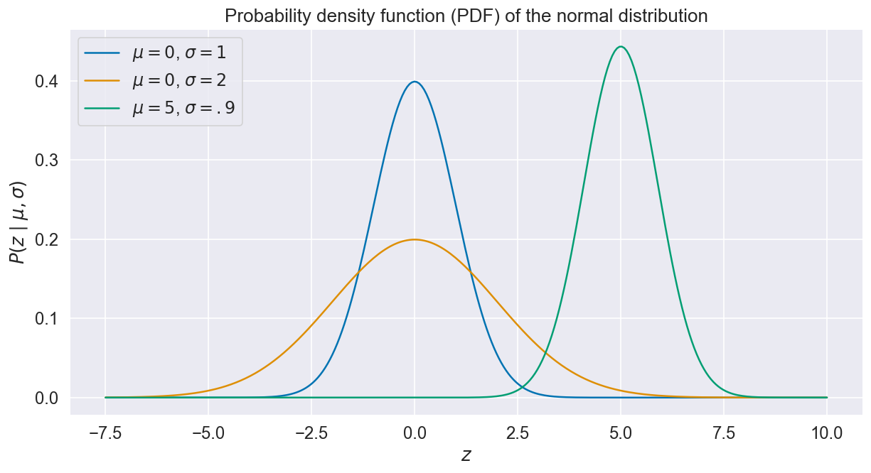
The normal distribution $\mathcal{N}$ with mean $\mu$ and standard deviation $\sigma$ is defined as follows:

$\tag{i} z \sim \mathcal{N}(\mu, \sigma) \iff P(z \mid \mu, \sigma) = \frac{1}{\sigma\sqrt{2\pi}} \cdot exp\left\{-\frac{1}{2}\left(\frac{z - \mu}{\sigma}\right)^2\right\}$

Here, “$\sim$” merely means “sampled from”, and $P(z \mid \mu, \sigma)$ is the probability density function (PDF), a quantity that determines the likelihood of a value $z$ given the distribution mean and standard deviation. Instances of Normal PDFs are shown below for various values of $\mu$ and $\sigma$.

Parametrizing the normal distribution

Let’s assume we are trying to model an outcome $y$ from a set of features $x$. In the classical, non probabilistic setting, our neural network is represented by a function $f$, which depends both on the input $x$ and the trainable parameters $\Theta$:

$y = f(x, \Theta)$

How can we turn this model into a probabilistic neural network?

• Looking back at the previous section, we can equate the prediction of our model with the distribution mean $\mu$: not withstanding uncertainty, $\mu$ is the most probable outcome.
• In turn, assuming a normal distribution is appropriate in this context, the standard deviation $\sigma$ is a good statistic to summarize the uncertainty surrounding our prediction.

Let $\mu(x, \Theta_1)$ and $\sigma(x, \Theta_1)$ be two sub networks with respective trainable parameters $\Theta_1$ and $\Theta_2$.

The mean network $\mu(x, \Theta_1)$ is nothing more than the original network $f$, i.e. the model prediction. The second network $\sigma(x, \Theta_2)$ is responsible for explicitly modeling uncertainty. From (i), we get:

$\tag{ii} y \sim \mathcal{N}\,[\,\mu(x, \Theta_1), \sigma(x, \Theta_2)\,]$

Note that in practice, $\Theta_1$ and $\Theta_2$ overlap, i.e. the two networks share their first few layers. (We’ll look at an in-depth example later on.)

We now have two sub-networks, with both shared and distinct parameters. We’d really like to train them jointly, using a single loss function.

The probability density function of equation (i) is an ideal candidate: the trick is to maximize the likelihood of observing $y$, which the PDF represents exactly.

It is best to take the logarithm of the PDF rather than dealing with the pesky exponential. Plus, PyTorch expects a function to minimize, so we are negating the quantity: the loss function is the negative log likelihood of observing $y$ given $x$, $\Theta_1$ and $\Theta_2$:

$\tag{iii} \mathcal{L} = \frac{1}{2}\left(\frac{y - \mu(x, \Theta_1)}{\sigma(x, \Theta_2)}\right)^2 + log\,\left\{\,\sqrt{2\pi}\cdot\sigma(x, \Theta_2)\,\right\}$

Notice how we recovered the square of difference term $(y - \mu)^2$ from the classic mean squared error, decorated with terms dependent on the standard deviation.

This is it, we have parametrized the normal distribution with a neural network and devised an appropriate loss function. Every input gets its own unique set of mean (prediction) and standard deviation (uncertainty) neatly calibrated from optimization of the PDF.

Enough theory, onward to the implementation.

Application: predicting cancer mortality rate

We’ll use data from the OLS Regression Challenge, where the goal is to predict cancer mortality rates in US counties based on a number of socio-demographic variables such as median age, income, poverty rate, unemployment rate, etc.

We won’t be discussing the dataset or data prep steps any further, but the code to reproduce is available on this jupyter notebook.

On to the implementation of the PyTorch model:

class DeepNormal(nn.Module):

    def __init__(self, n_inputs, n_hidden):
        super().__init__()

        # Shared parameters
        self.shared_layer = nn.Sequential(
            nn.Linear(n_inputs, n_hidden),
            nn.ReLU(),
            nn.Dropout(),
        )
        
        # Mean parameters
        self.mean_layer = nn.Sequential(
            nn.Linear(n_hidden, n_hidden),
            nn.ReLU(),
            nn.Dropout(),
            nn.Linear(n_hidden, 1),
        )
        
        # Standard deviation parameters
        self.std_layer = nn.Sequential(
            nn.Linear(n_hidden, n_hidden),
            nn.ReLU(),
            nn.Dropout(),
            nn.Linear(n_hidden, 1),
            nn.Softplus(),  # enforces positivity
        )
             
    def forward(self, x):
        # Shared embedding
        shared = self.shared_layer(x)
        
        # Parametrization of the mean
        μ = self.mean_layer(shared)
        
        # Parametrization of the standard deviation
        σ = self.std_layer(shared)
        
        return torch.distributions.Normal(μ, σ)

The bulk of the implementation should look familiar: network layers (including trainable parameters) are defined in the __init__ function, then the forward function pieces everything together.

A few specifics worth noting:

• The first hidden layer is shared and creates a common embedding.
• Next, computation branches out into mean and standard deviation sub-networks.
• The standard deviation branch ends with a softplus transformation to enforce positivity.
• The forward method outputs a Normal object parametrized by the output of both branches.

Moving on to the loss function:

def compute_loss(model, x, y):
    normal_dist = model(x)
    neg_log_likelihood = -normal_dist.log_prob(y)
    return torch.mean(neg_log_likelihood)

Commentary:

• As per the forward method above, calling the model returns a distribution object.
• This object provides a log_prob method. Its implementation is equivalent to equation (iii).
• An average over all inputs is returned.

Training can proceed just as with any other PyTorch model.

The normal distribution object provides mean and stddev attributes:

model.eval()
normal_dist = model(x)    # evaluate model on x with shape (N, M)
mean = normal_dist.mean   # retrieve prediction mean with shape (N,)
std = normal_dist.stddev  # retrieve standard deviation with shape (N,)

Goodness of fit after training:

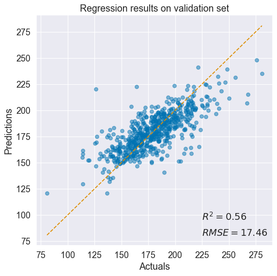
The model does a decent job at predicting cancer mortality rate.

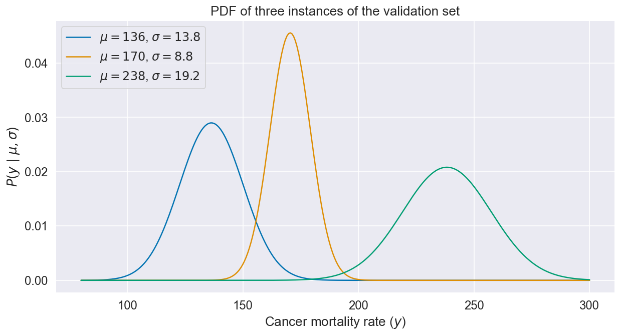
Distribution of the two model outputs $\mu$ and $\sigma$:

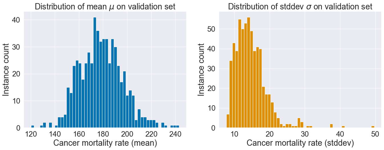
Different instances get different uncertainty profiles since $\mu$ and $\sigma$ both depend on $x$:

How good is our estimate of uncertainty?

One way to find out is to compare uncertainty to a measure of how surprinsing or unexpected an input is. Unexpected inputs should correlate with higher uncertainty (e.g. a self-driving car encountering a rare weather event).

For our purpose here, unexpectedness is measured as the average deviation from the median of an instance’s feature values. The most extreme the feature values, the more unexpected an instance.

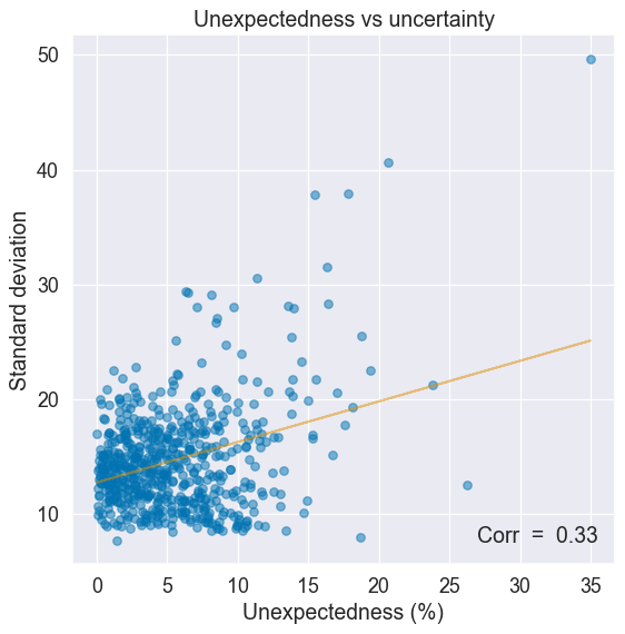
There is an upward trend: uncertainty tends to grow with less expected inputs, just as it should.

Take away

PyTorch distributions package provides an elegant way to parametrize probability distributions.

In this post, we modeled uncertainty using the Normal distribution, but there are a plethora of other distributions available for different problems.

Gist of this approach:

• Pick an appropriate probability distribution.
• Design a neural network to output one value per parameter in the target distribution.
• Jointly optimize these sub-networks using the probability density function as loss.

The benefit is an estimate of uncertainty around the model prediction, at the cost of a few extra layers.

This approach is easy and versatile — it is my go to method when I need a sense of uncertainty.

Full code is available here.